Evaluating robustness
With parameter sets generated from multi-omics data and enzyme kinetic databases, RobustNet constructs an ensemble of stochastic kinetic models, where each sampled parameter set defines one realization of the metabolic system. These ensemble models represent uncertainty in metabolic parameters and are used to simulate metabolic responses to engineering interventions, typically enzyme expression perturbations, and to evaluate metabolic robustness, i.e., whether and how likely the metabolic system can maintain a physiologically meaningful steady state following perturbation. Simulations are performed using a continuation-like method that directly solves steady-state sensitivity equations along the perturbation trajectory, thereby avoiding repeated and computationally expensive time-domain integrations from scratch after each perturbation step.
Simulating enzyme perturbations
Using the same E. coli model, assume that the parameter sampling procedure has already been completed and the returned samp_res stores sampled metabolite concentrations, enzyme concentrations, and kinetic parameters for ensemble model construction (see Parameterizing the model for more details). The evaluate_robustness can then be used to simulate perturbations of specified enzyme(s).
For example, a 10-fold overexpression of pyruvate dehydrogenase relative to its reference-state expression level can be simulated as follows:
[1]:
metab_sets = samp_res.sampled_metabolite_concentrations
enz_sets = samp_res.sampled_enzyme_concentrations
kparam_sets = pd.concat(
    (samp_res.sampled_kinetic_parameters, metab_sets),
    axis=1
)

model.load_parameter_sets(
    mconc_set=metab_sets,
    econc_set=enz_sets,
    kparam_set=kparam_sets
)
rob_res = model.evaluate_robustness(
    perturb_enzymes=['PDH'],
    fold_change=(1, 10),
    n_steps=300,
    n_models=1000,
    n_jobs=100
)
WARNING: AC, ETOH, FOR, GLC, LAC, O2 appear in rate expressions but not in the stoichiometric matrix. This likely means they are excluded or considered as unbalanced metabolites. When performing robustness analysis, they are treated as kinetic parameters, and their concentrations will not be simulated.
WARNING: Hcyt, Hper appear in the stoichiometric matrix but not in rate expression. They will be excluded from robustness analysis to maintain numerical stability.
INFO: Perturb enzyme PDH (1, 10)
Note: Sensitivities are not explicitly calculated for certain metabolites, such as end metabolites or metabolites that appear only in rate expressions as activators or inhibitors and do not participate directly as substrates or products in the stoichiometric network. Their concentrations are instead treated as regular kinetic parameters. To account for these metabolites, the input kparam_set should include both sampled kinetic parameter sets and sampled metabolite concentration sets
corresponding to these metabolites.
exclude_metabolites can be used to exclude metabolites from sensitivity analysis.
n_steps controls the number of integration steps used to solve the sensitivity equations. Larger perturbation ranges generally require higher n_steps values for improved numerical stability and smoother trajectories. Perturbation points can be either evenly spaced or logarithmically spaced by setting log_spacing.
The size of the ensemble used in robustness analysis is specified by n_models.
The robustness of the metabolic system can be evaluated from the probability of ensemble models remaining viable across the perturbation range, which can be visualized using:
[2]:
rob_res.robust_model_probability(out_dir=None, show_fig=True)
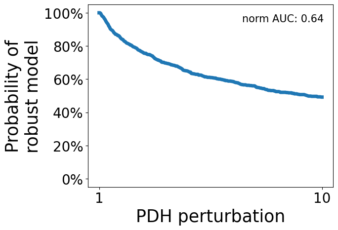
The robustness index (RI) provides a quantitative measure of system robustness and is defined as the normalized area under the survival probability curve across the specified perturbation range. RI ranges from 0 to 1, where lower values indicate a fragile metabolic system and higher values indicate stronger metabolic resilience against the specified perturbation.
[3]:
print(f'Robustness index: {rob_res.robust_index:.3f}')
Robustness index: 0.644
Below demonstrates the robustness under a 2-fold downregulation of the same enzyme.
[4]:
rob_res = model.evaluate_robustness(
    perturb_enzymes=['PDH'],
    fold_change=(0.5, 1),
    n_steps=300,
    n_models=1000,
    n_jobs=100
)
rob_res.robust_model_probability(out_dir=None, show_fig=True)
print(f'Robustness index: {rob_res.robust_index:.3f}')
WARNING: AC, ETOH, FOR, GLC, LAC, O2 appear in rate expressions but not in the stoichiometric matrix. This likely means they are excluded or considered as unbalanced metabolites. When performing robustness analysis, they are treated as kinetic parameters, and their concentrations will not be simulated.
WARNING: Hcyt, Hper appear in the stoichiometric matrix but not in rate expression. They will be excluded from robustness analysis to maintain numerical stability.
INFO: Perturb enzyme PDH (0.5, 1)
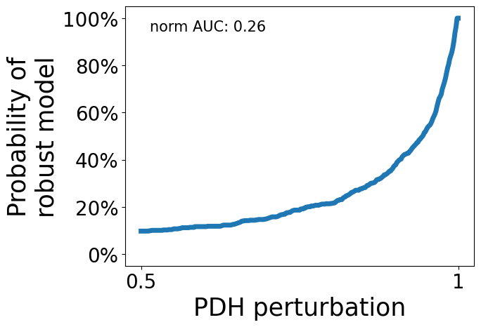
Robustness index: 0.257
The fold_change range must always include 1, corresponding to the reference state. If 1 is used as one of the bounds, the perturbation is simulated only in a single direction, representing either upregulation or downregulation as shown above. If the fold-change interval spans across 1, perturbations are simulated from the reference state toward both lower and upper bounds.
The following example demonstrates robustness analysis under up to 5-fold knockdown and 5-fold overexpression of the same enzyme.
[5]:
rob_res = model.evaluate_robustness(
    perturb_enzymes=['PDH'],
    fold_change=(0.2, 5),
    n_steps=300,
    n_models=1000,
    n_jobs=100
)
rob_res.robust_model_probability(out_dir=None, show_fig=True)
print(f'Robustness index: {rob_res.robust_index:.3f}')
WARNING: AC, ETOH, FOR, GLC, LAC, O2 appear in rate expressions but not in the stoichiometric matrix. This likely means they are excluded or considered as unbalanced metabolites. When performing robustness analysis, they are treated as kinetic parameters, and their concentrations will not be simulated.
WARNING: Hcyt, Hper appear in the stoichiometric matrix but not in rate expression. They will be excluded from robustness analysis to maintain numerical stability.
INFO: Perturb enzyme PDH (0.2, 5)
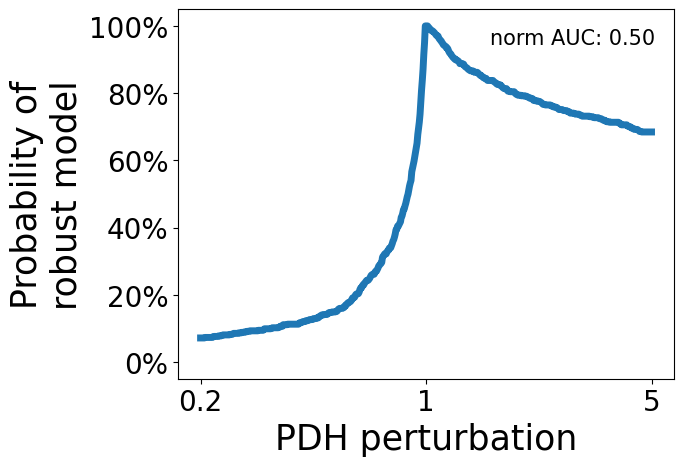
Robustness index: 0.499
Multiple-enzyme perturbations are also supported. For example, citrate synthase and 2-oxoglutarate dehydrogenase can be co-overexpressed with different fold-change ranges as follows:
[6]:
rob_res = model.evaluate_robustness(
    perturb_enzymes=['GlcPTS', 'PDH'],
    fold_change={
        'GlcPTS': (1, 2),
        'PDH': (1, 5)
    },
    n_steps=300,
    n_models=1000,
    n_jobs=100
)
rob_res.robust_model_probability(out_dir=None, show_fig=True)
print(f'Robustness index: {rob_res.robust_index:.3f}')
WARNING: AC, ETOH, FOR, GLC, LAC, O2 appear in rate expressions but not in the stoichiometric matrix. This likely means they are excluded or considered as unbalanced metabolites. When performing robustness analysis, they are treated as kinetic parameters, and their concentrations will not be simulated.
WARNING: Hcyt, Hper appear in the stoichiometric matrix but not in rate expression. They will be excluded from robustness analysis to maintain numerical stability.
INFO: Perturb enzyme GlcPTS (1, 2), PDH (1, 5)
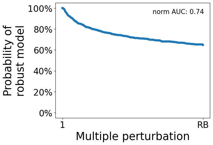
Robustness index: 0.742
Simultaneous knockdown and overexpression of different enzymes can also be simulated, as illustrated below.
[7]:
rob_res = model.evaluate_robustness(
    perturb_enzymes=['GlcPTS', 'PDH'],
    fold_change={
        'GlcPTS': (1, 2),
        'PDH': (1, 0.2)
    },
    n_steps=300,
    n_models=1000,
    n_jobs=100
)
rob_res.robust_model_probability(out_dir=None, show_fig=True)
print(f'Robustness index: {rob_res.robust_index:.3f}')
WARNING: AC, ETOH, FOR, GLC, LAC, O2 appear in rate expressions but not in the stoichiometric matrix. This likely means they are excluded or considered as unbalanced metabolites. When performing robustness analysis, they are treated as kinetic parameters, and their concentrations will not be simulated.
WARNING: Hcyt, Hper appear in the stoichiometric matrix but not in rate expression. They will be excluded from robustness analysis to maintain numerical stability.
INFO: Perturb enzyme GlcPTS (1, 2), PDH (1, 0.2)
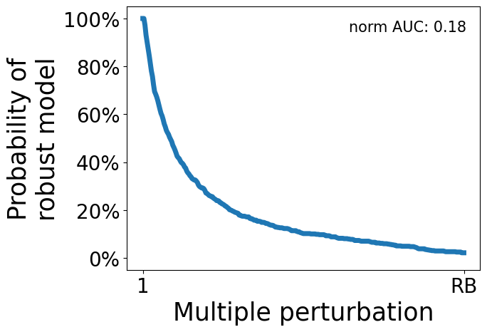
Robustness index: 0.181
In general, perturbations involving arbitrary combinations of enzymes and expression fold changes are supported.
Inspecting metabolic responses
The simulation results can be further analyzed to investigate metabolic responses, including changes in steady-state metabolite concentrations and metabolic fluxes following perturbation.
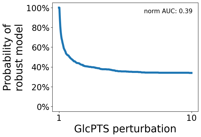
Below, we demonstrate a 10-fold overexpression of GlcPTS as an example.
[8]:
rob_res = model.evaluate_robustness(
    perturb_enzymes=['GlcPTS'],
    fold_change=(1, 10),
    n_steps=300,
    n_models=1000,
    n_jobs=100
)
WARNING: AC, ETOH, FOR, GLC, LAC, O2 appear in rate expressions but not in the stoichiometric matrix. This likely means they are excluded or considered as unbalanced metabolites. When performing robustness analysis, they are treated as kinetic parameters, and their concentrations will not be simulated.
WARNING: Hcyt, Hper appear in the stoichiometric matrix but not in rate expression. They will be excluded from robustness analysis to maintain numerical stability.
INFO: Perturb enzyme GlcPTS (1, 10)
[9]:
rob_res.robust_model_probability(out_dir=None, show_fig=True)
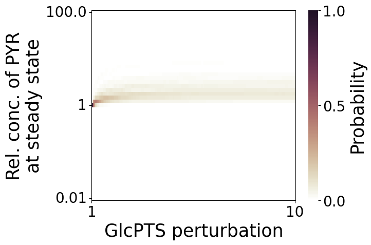
Metabolite responses can be visualized using the metabolite_sensitivity method (alias bifurcation_diagram).
We inspect the steady-state pyruvate concentration relative to its reference-state level in response to this perturbation.
[10]:
rob_res.metabolite_sensitivity(
    out_dir=None,
    kind='sample',
    metabolites=['PYR'],
    show_fig=True
)
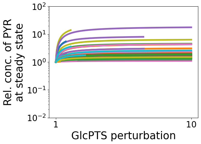
Here metabolite response trajectories are visualized using sampled trajectories from ensemble models, where the number of displayed trajectories can be controlled through n_sets. Trajectories that terminate early indicate the occurrence of bifurcations or the emergence of non-physiological metabolite concentrations during perturbation. Alternatively, setting kind to “stats” displays a probability-density heatmap summarizing the responses across all models.
[11]:
rob_res.metabolite_sensitivity(
    out_dir=None,
    kind='stats',
    metabolites=['PYR'],
    show_fig=True
)
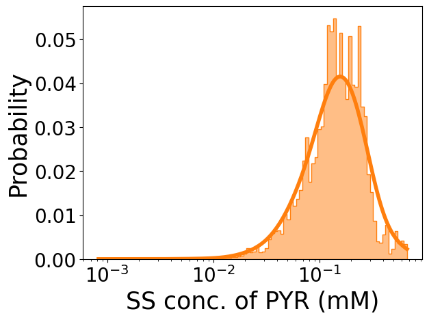
The metabolite_distribution method visualizes the distribution of possible pyruvate concentrations throughout the perturbation process.
[12]:
rob_res.metabolite_distribution(
    out_dir=None,
    metabolites=['PYR'],
    show_fig=True
)
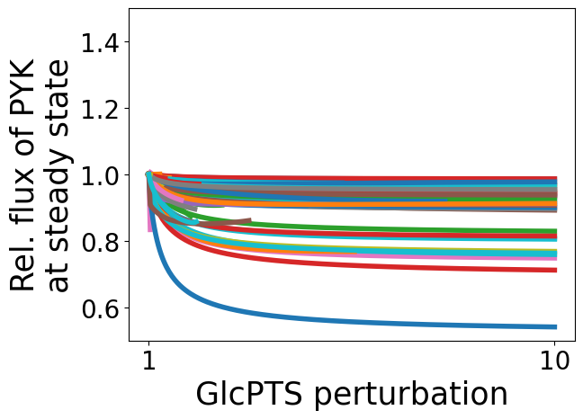
In addition to metabolite concentrations, steady-state metabolic fluxes after perturbation can also be analyzed. The following example demonstrates how flux_sensitivity visualizes changes in pyruvate kinase flux relative to its reference-state value under perturbation.
[13]:
rob_res.flux_sensitivity(
    out_dir=None,
    kind='sample',
    reactions=['PYK'],
    show_fig=True
)
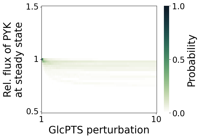
[14]:
rob_res.flux_sensitivity(
    out_dir=None,
    kind='stats',
    reactions=['PYK'],
    show_fig=True
)
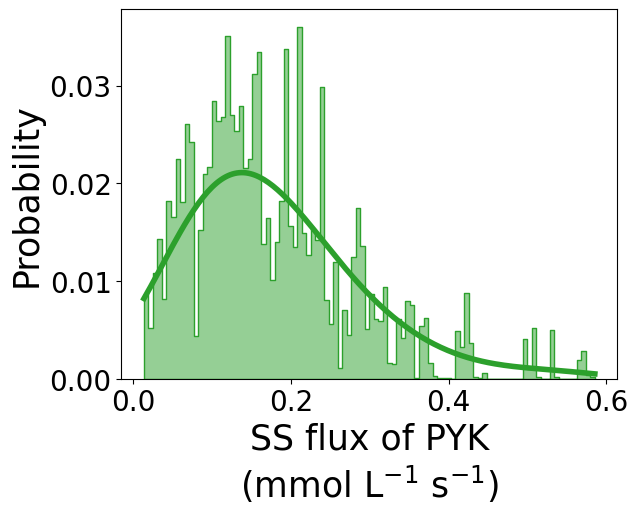
Similarly, the distribution of absolute flux values carried by the reaction during perturbation can be visualized as:
[15]:
rob_res.flux_distribution(
    out_dir=None,
    reactions=['PYK'],
    show_fig=True
)