Parameterizing the model

Multi-omics data, including fluxomics, metabolomics, and proteomics, together with enzyme kinetic databases such as BRENDA and SABIO-RK, as well as thermodynamics resources such as eQuilibrator, provide rich sources of information for parameterizing the kinetic model. However, these measurements are typically collected from different studies and experimental conditions and inherently contain noise and uncertainty. As a result, directly combining them often fails to produce a kinetically consistent model in which the mechanistic rate laws and steady-state constraints are simultaneously satisfied.

RobustNet adopts a Bayesian framework to infer feasible model parameters (posterior distributions) that remain close to the experimentally measured data (prior distributions) while trying to maintain consistency with the kinetic equations and feasible steady states.

Estimating the reference flux distribution

The first step is to estimate the reference-state flux distribution, which represents the steady-state metabolic fluxes before enzyme perturbation. These fluxes are typically obtained from isotope-assisted metabolic flux analysis (MFA). Our previously developed package, FreeFlux, can be used for this purpose.

Because the metabolic network used for MFA may differ from the kinetic network constructed in RobustNet, a calibration step is required to derive a flux distribution that both satisfies mass balance in the current network and remains close to the MFA estimates.

This step can be performed as follows:

import pandas as pd
from robustnet import Model

MODEL_FILE = '../../models/e_coli/e_coli_model.xlsx'

model = Model('ecoli')
model.read_from_file(MODEL_FILE)

FLUXOMICS = '../../models/e_coli/measured_fluxes.xlsx'
FLUX_BOUNDS = '../../models/e_coli/flux_bounds.xlsx'

flux_data = pd.read_excel(FLUXOMICS, header=0, index_col=0)
flux_bounds = pd.read_excel(FLUX_BOUNDS, header=0, index_col=0)

model.load_priors(
    'fluxomics',
    data=flux_data.iloc[:,0],
    std=flux_data.iloc[:,1],
)
fit_res = model.estimate_reference_fluxes(
    bounds={rxn: tuple(row) for rxn, row in flux_bounds.iterrows()},
    optimizer='scipy',
    method='COBYQA',
    tol=1e-8
)

Note: Intracellular metabolite and enzyme concentrations are typically expressed in mM. To maintain unit consistency and appropriate numerical scaling, fluxes in RobustNet are represented in units of mmol L\(^{-1}\) s\(^{-1}\).

Additional flux bounds can be provided to constrain the estimated fluxes and specify reaction directionality. For example, a lower bound greater than 0 enforces a forward-only reaction and an upper bound less than 0 enforces a reverse-only reaction as defined by the reaction direction in the model.

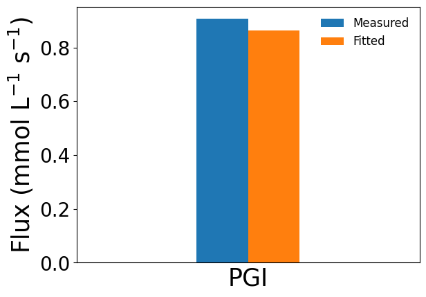
The estimated reference fluxes and their uncertainties can be accessed through the estimated_fluxes and estimated_flux_errors attributes of the returned FluxFitResults object. Comparison between the calibrated fluxes and the original MFA estimates can be visualized using the provided plotting function (using glucose-6-phosphate isomerase as an example).

fit_res.plot_simulated_vs_measured_fluxes(
    out_dir=None,
    reactions=['PGI'],
    show_fig=True
)

Generating model parameter sets

The calibrated reference flux distribution is then integrated with metabolomics, proteomics, and enzyme kinetic data to generate ensemble model parameter sets. This step is performed by sampling from the posterior distributions of metabolite concentrations, enzyme concentrations, and kinetic parameters.

The following example demonstrates this procedure.

METABOLOMICS = '../../models/e_coli/measured_metabolites.xlsx'
PROTEOMICS = '../../models/e_coli/measured_enzymes.xlsx'
KINETIC_PARAMETERS = '../../models/e_coli/measured_kinetic_parameters.xlsx'

metab_data = pd.read_excel(METABOLOMICS, header=0, index_col=0)
enz_data = pd.read_excel(PROTEOMICS, header=0, index_col=0)
kparam_data = pd.read_excel(KINETIC_PARAMETERS, header=0, index_col=0)

model.load_priors(
    'reference_fluxes',
    data=fit_res.estimated_fluxes,
    std=fit_res.estimated_flux_errors
)
model.load_priors(
    'metabolomics',
    data=metab_data.iloc[:,0],
    std=metab_data.iloc[:,1],
)
model.load_priors(
    'proteomics',
    data=enz_data.iloc[:,0],
    std=enz_data.iloc[:,1],
)
model.load_priors(
    'kparameters',
    data=kparam_data.iloc[:,0],
    std=kparam_data.iloc[:,1]
)
samp_res = model.generate_parameter_sets(
    alpha=None,
    n_tunes=5000,
    n_samples=2000,
    n_chains=10,
    n_jobs=10
)

Note: Metabolomics and proteomics data are expected in units of mM (cell volume-based). For kinetic parameters, catalytic constants have units of s\(^{-1}\), Michaelis, activation, and inhibition constants have units of mM, and equilibrium constants are dimensionless.

During posterior sampling, the alpha argument defines a tunable coefficient that controls the tradeoff between consistency with experimental measurements and feasibility of the kinetic model.

• A smaller alpha keeps the posterior distributions closer to the original omics measurements and generally makes sampling easier, but the resulting kinetic model may be less balanced.

• A larger alpha enforces stronger consistency between the kinetic equations and the reference steady state, but may lead to more difficult sampling and reduced convergence efficiency.

By default, alpha is set to the geometric mean of the inverse variances of the reference fluxes.

n_tunes is directly passed to the PyMC samplers and controls the number of tuning (burn-in) iterations used to stabilize sampling before posterior samples are collected. The total number of posterior samples is determined by both the number of sampling chains specified by n_chains and the number of samples drawn per chain specified by n_samples.

After sampling is completed, all results are received by samp_res. In particular, sampled kinetic parameter sets can be accessed through the sampled_kinetic_parameters attribute.

samp_res.sampled_kinetic_parameters.sample(5)

	Ka_ACCOA_vPPC	Ka_FBP_vPPC	Ka_FBP_vPYK	Ka_PEP_vFBPase	Keq_vACK	Keq_vACON	Keq_vADK	Keq_vAKGDH	Keq_vALCD	Keq_vALDDH	...	kcat_vPTA	kcat_vPYK	kcat_vRPE	kcat_vRPI	kcat_vSDH	kcat_vSUCOAS	kcat_vTAL	kcat_vTKT1	kcat_vTKT2	kcat_vTPI
10973	1.870129	0.870527	1.747532	2.243964	337.527424	0.073662	0.699464	155582.867178	1192.781793	0.491528	...	21.905336	124.891760	2.109956	2064.644968	76.213010	2.473156	13.864075	2.043599	1.760774	8741.377981
7099	2.332932	1.868009	0.978254	2.331784	322.006271	0.033219	0.945926	123754.968077	1026.579617	0.190596	...	131.290824	138.561988	1.863342	273.485551	59.245313	1.070354	12.369193	0.937129	1.461572	7178.409988
6569	2.010493	1.770139	0.833338	2.076259	141.966629	0.115442	0.839103	362922.022172	1356.087648	0.127495	...	155.345317	134.760783	2.146779	2355.050995	132.490001	3.681403	15.224663	0.254971	2.363003	9332.960377
9233	2.198546	1.933340	1.249352	2.111623	229.801055	0.081238	1.003101	185048.884845	1572.620443	0.225697	...	31.319926	153.433054	1.755173	586.469550	86.098486	2.388448	13.255742	1.460273	1.749851	7113.498239
7963	2.387464	1.557875	3.141863	3.601756	261.003044	0.160908	1.022405	103608.127097	1432.528746	0.297042	...	113.045903	153.958044	2.227516	311.411164	58.020611	1.738744	11.246085	2.944525	2.777271	7547.605797

5 rows × 351 columns

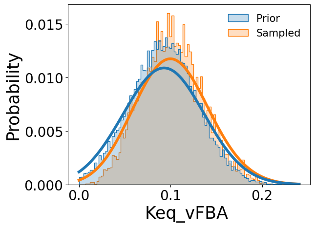
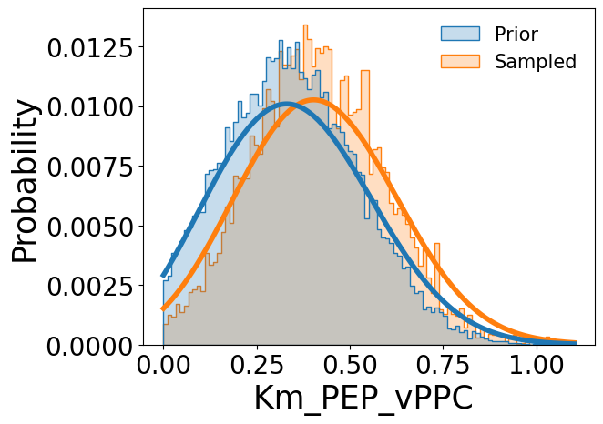
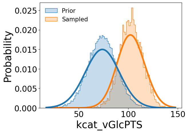
Comparisons between the prior distributions and sampled posterior distributions can be visualized using the provided plotting utility, illustrated here using the catalytic constant k\(_{cat}^{GlcPTS}\), Michaelis constant K\(_{m}^{PEP,PPC}\), and equilibrium constant K\(_{eq}^{FBA}\):

samp_res.plot_sampled_vs_prior_kinetic_parameters(
    out_dir=None,
    parameters=['kcat_vGlcPTS', 'Km_PEP_vPPC', 'Keq_vFBA'],
    show_fig=True
)

Similarly, sampled metabolite concentration sets can be accessed through

samp_res.sampled_metabolite_concentrations.sample(5)

	AC	ACALD	ACCOA	ACETP	ADP	AKG	AMP	ATP	BPG	CIT	...	PYR	Pi	R5P	Ru5P	S7P	SUC	SUCCOA	UQ	UQH2	Xu5P
9932	0.210686	0.181244	0.302144	0.186986	0.030406	0.052820	0.008098	0.479109	0.137904	0.147553	...	0.054040	0.147472	0.018113	0.045438	0.145702	0.172249	0.132912	0.147945	0.141645	0.097859
7854	0.216531	0.125369	0.312520	0.150798	0.052235	0.045836	0.005128	0.510380	0.184664	0.196658	...	0.056460	0.145168	0.024162	0.109934	0.170378	0.140536	0.174965	0.200266	0.139823	0.179706
15282	0.210595	0.108958	0.337574	0.139802	0.055148	0.059934	0.005603	0.496219	0.177995	0.100588	...	0.072680	0.157538	0.029852	0.024523	0.112865	0.213476	0.102343	0.084586	0.135467	0.219680
276	0.202213	0.180576	0.287823	0.096652	0.083652	0.063701	0.006530	0.476595	0.177534	0.114668	...	0.046049	0.091807	0.018890	0.113220	0.174743	0.144751	0.105163	0.112118	0.257921	0.093595
6274	0.195270	0.233839	0.314113	0.225211	0.042064	0.059626	0.006866	0.529823	0.074897	0.216247	...	0.144874	0.156079	0.015216	0.085632	0.076764	0.125076	0.185114	0.142033	0.195642	0.183659

5 rows × 50 columns

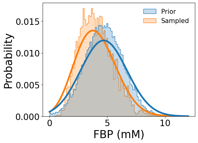
and compared with the prior metabolomics data (using fructose 1,6-bisphosphate as an example).

samp_res.plot_sampled_vs_prior_metabolites(
    out_dir=None,
    metabolites=['FBP'],
    show_fig=True
)

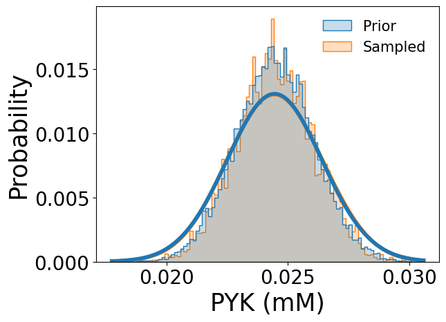
Sampled enzyme concentration sets are available through sampled_enzyme_concentrations, and comparisons with the prior proteomics data can be visualized (using pyruvate kinase as an example) as follows:

samp_res.sampled_enzyme_concentrations.sample(5)

	ACK	ACON	ADK	AKGDH	ALCD	ALDDH	ATPSyn	COX	CS	EDA	...	PPS	PTA	PYK	RPE	RPI	SDH	SUCOAS	TAL	TKT	TPI
1219	0.002922	0.038921	0.007545	0.009021	0.005966	0.006592	0.009701	0.001923	0.016836	0.008288	...	0.003619	0.003650	0.026954	0.007377	0.001651	0.004758	0.015840	0.019835	0.012376	0.005850
18685	0.003086	0.043500	0.008532	0.009250	0.006752	0.006218	0.009592	0.001733	0.016289	0.009758	...	0.003315	0.003463	0.023613	0.008305	0.001588	0.004434	0.014752	0.022703	0.013093	0.007637
15394	0.003669	0.050088	0.009360	0.008551	0.007302	0.006157	0.009723	0.002148	0.015850	0.009089	...	0.003443	0.003760	0.023940	0.008740	0.001465	0.003998	0.014591	0.022720	0.012212	0.007396
6000	0.003094	0.047729	0.008681	0.008357	0.008051	0.006331	0.009771	0.001866	0.017154	0.008673	...	0.003319	0.004492	0.025234	0.007138	0.001584	0.004128	0.015617	0.019959	0.013493	0.007629
9147	0.003227	0.045774	0.007356	0.009303	0.007498	0.006192	0.009635	0.001931	0.017013	0.008218	...	0.003567	0.003756	0.021409	0.008609	0.001349	0.004255	0.014663	0.015976	0.011786	0.006127

5 rows × 48 columns

samp_res.plot_sampled_vs_prior_enzymes(
    out_dir=None,
    enzymes=['PYK'],
    show_fig=True
)

The full sampling trace is stored in samp_res.trace, which returns an arviz.InferenceData object. This enables direct compatibility with the analysis tool provided by ArviZ.